Mini Project- Analysis of the Declining Bat Population in Select Counties of Wisconsin

Introduction:

I chose the declining bat population in Wisconsin as my project.  I wanted to research why this is happening and if there are any factors contributing to this.  I chose to see if this decline was based on certain criteria.  The study question is, is the bat population declining in Wisconsin, and if so where and is there something responsible for it.  My hypothesis is that the decline is due to many factors but the most important one is that the increased amount of pesticides are part of the problem and maybe the biggest part.  In my results section I included maps that show that the more pesticides in an area that is where the decline is the greatest.  Instead of finding the most suitable areas for bats, I chose to research the areas where there was a decline. 

Methods:

I used a series of  analysis done by the  Wisconsin Department of Natural Resources to show the amount of bats in each of the counties that had enough data to go on.  In the information I received from the DNR, there were many counties that did not have enough data to use in my analysis, namely Stonefield, Dodge, and Yellow Lake.  These counties only had data for one year or for only a few detection sites and not significant enough to map or analyze.  The counties chosen to analyze to see if there has been a decline in the population of bats are as follows, Grant, Iowa, Lafayette, Trempealeau and Door Counties.

First I analyzed he data from the DNR, then I decided to see if my hypothesis was right that the bat population in Wisconsin is declining.  I did this by adding all the bat radar analysis.  On the nights the researchers went out, they used the counts of bats to see where the bats were and how many.  The researchers went out at least 10 times per site and some other sites they had more visits.  Because of this I normalized the data.  I chose the most recent data provided and did an analysis of 2014 and 2015 to see if there was a difference.  I also used a buffer of 500 feet away from a major road or interstate to see if the bats are staying closer to roads that have trees or it they are staying near trees in the wooded areas.  I then used the Euclidean distance to see if the distance between two points and counted in metric space, I selected the distance from the center of the cities of Wisconsin.  The next tool I used was intersect, I intersected all the buffer zones. 

First is the map I created in ArcGIS with the above counties and the counts of the bats for 2014 and 2015, it shows that the population did in fact decrease.  The map also shows that there are not many bats near larger cities and where many major interstates are present.  If you notice in maps 1 and 2, of Wisconsin Bat Population of 2014 and 2015, the area on the south eastern part of the state has very large populations and there are not bat hibernation cites in this area.  This is also true for the other counties that bat population has been counted in.  Bats tend to be in areas of less human traffic.  The below map shows that the population of bats decrease in Lafayette and Door Counties, there was a small decrease in Iowa county and Grant increased. This increase in Grant County could be due to the amount of increase traffic in Lafayette county or it could be the pesticide use, or many other factors.  The map clearly shows that there is a decrease of over 1,000 bats in Lafayette County. 

Maps 1 and 2:  Shows increase of bat population.  2015 map includes cities of Wisconsin for emphasis. 

 Next, I created a buffer of 500 feet from roads so we could see the if this played a role in the amount of bats in an area.

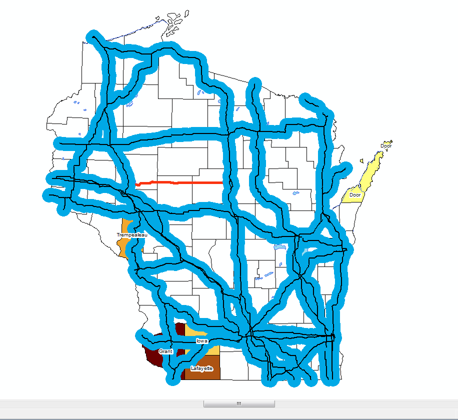
Map 3:  Buffer zones of 500 feet from major roads. 






 

This map shows the buffer zones and there are no major roads that go through Door County that would make this an issue for bats, the majority of the county of Lafayette is not in the buffer zone yet man of the bats migrated to Grant where there are more roads which leads me to believe that there is another variable affecting the population.

The next tool used was the Euclidean Distance and I chose to use it from the center of a city in Wisconsin.  Below is a map of the areas and how far from the city most of the bats are, if you notice at the bottom left or southwestern part of the image, it shows the distance from the center on Grant, Iowa and Lafayette Counties are not near the center of bigger cities.  Bats need trees or caved areas to live in which are not usually located near large cities. 

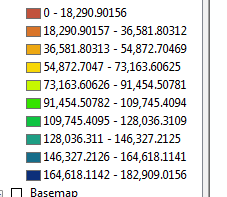
Figure 4: Euclidean Distance from Wisconsin cities. 

 

  



 

 

Map 4:  2005 Cropland layer map from the USGS website and cropscape. 

The above map was taken from the USGS website from the National Agricultural Statistics Service.  It displays in dark red the areas where the most pesticides were used.  If you see that this map is from 2005 and the United States uses far more now that before, the focus area, namely Lafayette County is covered in red and that is an area where the population has declined.  This is just another added part of the puzzle to show that there may be a high correlation between the two. 

 

 

Results:

 

The results were just as I thought with the creating a map in ArcMap with the Excel files I used from the WI DNR.  The bat population is declining in the focus area counties, also bats like to stay away from highways and busy cities.  If there is more development of urban areas near bat hibernation cites, the population can further decline.  The maps I provided did show exactly what I wanted them to.

 

 

Evaluation: 

 

This project was much harder than I thought, I had to wait a very long time to get the data and even longer for it to get analyzed so I could use it and make shapefiles for my maps.  I also had a hard time with all of the tools and had to re-run them a few times.  I put in too many variables to do the project properly.  I should have just stuck to where bats are located and why instead of doing the decline, reasons for it and introducing pesticide use.  I chose too many things to discuss and analyze therefore making my project not as understandable and not as easy to do.  It took me such a long period of time to analyze the data to see what I could and couldn't use.  That was time I could have used doing other parts of this assignment.  I had many challenges while doing this assignment because I had too many ideas and too many things involved in the results.  I  would change the whole entire outlook and I would have analyzed other counties in the U.S. not Wisconsin as the Wisconsin DNR does not have much data on the bats and they do not consider bats to be very important as diseases such as White-Nose Syndrome have not hit Wisconsin very hard, doing research on another county that has more data and more problems, then they would also have more information.  I also went out with Chris Floyd to collect data in Eau Claire but since there was so little data and the DNR said that they would need a few months to get the data we collected back to me from the radar collection. I had no idea that this would take that long.  I just over thought the whole thing and I really am not happy with the overall results except for the fact that the counties that use the most pesticides had the most decline in the bat population.  I just don't think overall I had enough information to do what I wanted with the project. 

 

 

References:

 

USGS Wisconsin Pesticide Maps

 

John. P. White, Wisconsin Department of Natural Resources

Lab 5 Vector Processing and Pyton Scripting.

Objectives: For Lab 5 there were a few objectives. First vector processing, the second part of the lab will be python scripting in part 2.    
Part 1:  Objective 1:  
Q1: Marquette_bear_study is a database. 
Q2: bear_management_area and landcover are data sets and shapefile.  
The objectives were to map a GPS MS Excel file of black bear locations in Michigan, to determine the forest types where black bears are found in central Marquette County, Michigan based on GPS locations of black bears, to determine if bears are found near streams, to find suitable bear habitat based on two criteria, to find all areas of suitable bear habitat within areas managed by the Michigan DNR, to eliminate areas near urban  lands, generate cartographic output, and to generate a digital data flow model of the procedures used to determine suitable bear habitat in Marquette County, Michigan. 

 Methods: The first thing to do was to add the bear locations as an XY event theme.  The best way to do this is to go to the File menu in ArcMap and choose add data and choose add XY data.  When the window pops up choose bear_location_geo$ from file folder and choose point_x for x field and point_y for y field.
Choose edit and choose NAD_1983_Hotline_Oblique_Mercator_Azimuth_Natural_Origin and click ok and ok again.  The bears should appear as points in ArcMap.  Once they are mapped export to bring them into your geodatabase as a feature class which has the ID number of the bear and the land cover type in which is was found in the attribute table. I then named the new feature class bear cover. 

Using the data found the 3 best habitat types. 
Q4a:  Habitat 1:  Evergreen Forest Land
Q4b:  Habitat 2:  Forested Wetlands
Q4c:  Habitat 3:  Mixed Forest

Objective 3:




 Add all the feature classes within the bear_management_area feature dataset to a data frame and arrange them properly. Then change the symbology for landcover layer so that  “minor type” field is able to be seen.  Then new landcover and bear locations should be intersected to create the bear cover feature layer.  Then use summarize to find out which are the top 3 habitats that bears are found in. Take bear locations and use select by locations to select areas that are within 500 meters of a stream when there GPS location was collected.  There were 49 out of 60 or 81.67 % of bears were found within 500 meters of a stream. 
I find this area to be suitable for bears due to the fact that the area selected is near streams and wooded areas away from the urban areas.  If 49 out of 60 bears are located there, then I would say that it a good representation of a good habitat for bears. 

Objective 4:

To find suitable areas of bear habitat by first using the select by attributes tool to select the 3 land types that bears were found in most and name it bear habitat. .  Then intersect the bear habitat and the bears found within 500 meters of a stream.  Then the dissolve tool is used to get rid of the polygon shapes that are found from more than one layer being combined.

Objective 5:

Next, add in the Michigan DNR data called DNR Management from the file.  To find suitable bear habitat that is located on the DNR management lands.  Use the intersect tool to intersect the habitat with the DNR management feature class to find a location within the DNR lands and then dissolve  to make the polygons solid and without features within polygons (Q8).

 

To find an area that is away from the urban environment use select by attribute to determine the urban areas so as to stay away from them.  Then use the buffer tool to buffer out a 5 kilometer area from urban areas.  Then dissolve the buffer so that there is one solid buffer.  Finally use erase so that only the best possible locations are available.

Results:  The first image is of the data flow model used to help follow along with what was done for methods.  The second image is of the map made with the best possible locations available.

Figure 1: Data Flow Model resulting in the best possible locations for a bear habitat. 

Figure 2:  Suitable Bear Habitat, Marquette, Michigan, notice the light green inset of the study area. 

The above map shows the areas that are ideal for bear habitat in pink, they are located near streams and have the attributes for proper living conditions for bears.  The dots are where bears are located and the red is where it is not suitable for bears. 

Discussion:
It is interesting that the areas in red that were not suitable for bear habitat did not have any bears in that area according to the data given, they were only close to the red in one area of the map located on the southwestern part of the map.  Also, the areas that are suitable for bears had a great deal of bears in the areas.  There were areas suitable that did have any bears in that area according to the data. This study area had a lot of areas suitable for bears. 

Part 2:  Introduction to Python Scripting

Introduction:

The objective of this lab is to learn how to use Python Scripting using ArcGIS with the python window and to explore the functionalities to run tools by writing scripts. 

Section 1: 

Objective is to find suitable areas for the development of tourist resorts.  The Wisconsin Department of Tourism wants to find areas within the state that have high potential for the establishment of suitable resorts.  The resorts should be within 10 miles from the city and 5 square miles in area.

First, I opened ArcMap and opened a new map.  I created a new map and I added the following features to my map, WI_Cities, Interstates, Lakes, an d Counties, then I clicked the python window to begin.  I then proceeded with the instructions to make a 10 mile buffer. 

Figure 1:  Buffer distance of 10 miles of a city. 

After typing in the codes, I pressed F2 to check for errors and there were none present, then I executed the command. 

Next, find the lakes that are greater than 5 square miles by writing a code to select the attribute. 

Figure 2: Lakes greater than 5 square miles. 

I had some trouble with this one but got it to work after some trial and error to make sure I had it written exactly right the last time I tried it. Final result is the last command. 






Figure 3:  Best Locations for Lakeside Resort Buffer

Section 2:  Modeling air pollution impact zones

Wisconsin EPA is interested in the assessment of potential impact zones for nitrous oxide and other air pollutants from automobiles near the interstates in Wisconsin and the human and ecosystem health. 

The criteria for air pollution impacts:  The Wisconsin EPA has determined that areas within six miles of an interstate have potential for air pollution problems with the impacts reducing the farther one is from an interstate.  The WI EPA wants you to develop an index model that will show six zone of potential air quality problems within a one mile interval. 

I created a multiple ring buffer.

Figure 4: Multiple Ring Buffer

Figure 5:  Interstate Multiple Ring Buffer Map with Cities. 

 

Figure 6: Zoomed in of Multiple Buffers to show values. 

 

Lab 3 Downloading and mapping GIS Data

 



 



Introduction:

 

The goal of this lab assignment is to learn how to obtain GIS data and other stand alone data to be used in a GIS project.  It also is intended to learn how to use the U. S. Census Bureau's website to acquire information for this purpose. 

 

Methods:

 

First I downloaded the 2010 U. S. Census Data from the U. S FactFinder webpage (total population).  I downloaded the shapefile for the 2010 Census boundaries.  I then joined the data to the shapefile.  I then made a map of the 2010 Housing  Population.  I made the maps and then I went to Properties, Symbology, then labels to make the numbers easier to understand by taking out many of the zeroes and rounding the numbers to make the legend understandable.  I chose colors that were easy to see and read so the information was the same in both maps with the regards to color gradient.  

 

 

Map 1:  2010 Total Population Census Data (pink).
This map shows the total population of Wisconsin in 2010.  It shows which counties are more populated than others and if you know anything about Wisconsin the dark pink highlighted counties are where the two largest Milwaukee and Madison are located. 

Map 2: (Green)  I chose the housing population.  It shows similar results that the most populated counties also have the most housing units occupied.  The two darkest green ones are where Milwaukee and Madison are located.  The large dark green county (large block in the southern middle, closest to the bottom is Dane County  and the Milwaukee County is located on the Eastern most the state. 

In both maps above, Marathon County, Brown and Outgamie County and Winnebago counties also have a larger population of people and housing.  The two categories are very similar in the results as the total population would need housing so these results have a strong correlation to each other. 

I saved all the information in my folder and on GIS. 

Bogstad Lab 4 Blogpost

Lab 1

The purpose of this lab is the understand Coordinate Systems and Map projections.  The goal is of this lab is to understand the differences between projected and geographic coordinate systems and how to apply then to our GIS projects.  Additionally, to find and identify errors in GIS data.  Then to re-project the data to be used in GIS. 

The objective is to build data frames displaying feature data of the world in different projections.  In this exercise we will change the projection for Wisconsin and create a map using the appropriate projection. 

First, I downloaded or unzipped the data file and saved it to my personal folder in the Q drive.  Then I opened ArcMap and set up all the files to save in lab 1.  Next, I set up the world predefined projections data frame.  I then added the country and geogrid to ArcMap.  I then changed the legends for each of the shapefiles to desirable colors that made it easier to read the maps.  I then set up the Geographic Projection.  I selected the appropriate coordinate system and then saved my map.  I saved it under my lab exercises and as an mxd.

Next, I build another data frame, I followed the same path to do this but used Mercator Projection.  I also changed all the symbols again.  After this I created three more coordinate systems, Sinusoidal, Equidistant-Conic and Miller Cylindrical.  I tried using colors that are pleasing to the eye and that were easily distinguished from other colors. 

 
This is a screen shot of the map coordinates and layouts that I chose. I made the maps large enough to be readable.

Next, I created a data frame for the Wisconsin data.  I inserted a new data frame and named it UTM  and added it to the map.  I then created a new shapefile for the states layer and I selected Wisconsin and highlighted it and exported it to my map.  I then changed the symbolization and set the data frame coordinate system to UTM,NAD1983,Zone16N.

I then did some trial and error to see how the projections looked.  I changed the projected coordinate system to North American Lambert Conformal Conic. 

Next, I created a map containing all of the seven data frames I created.  I resized them to look for conformed.  I then labeled them and organized them in a landscape view.